Figure
1.
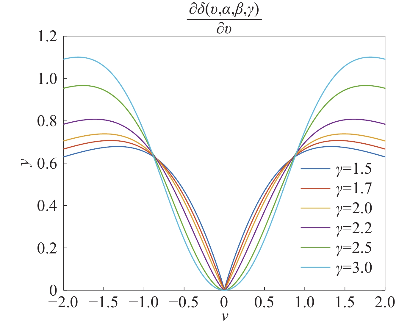
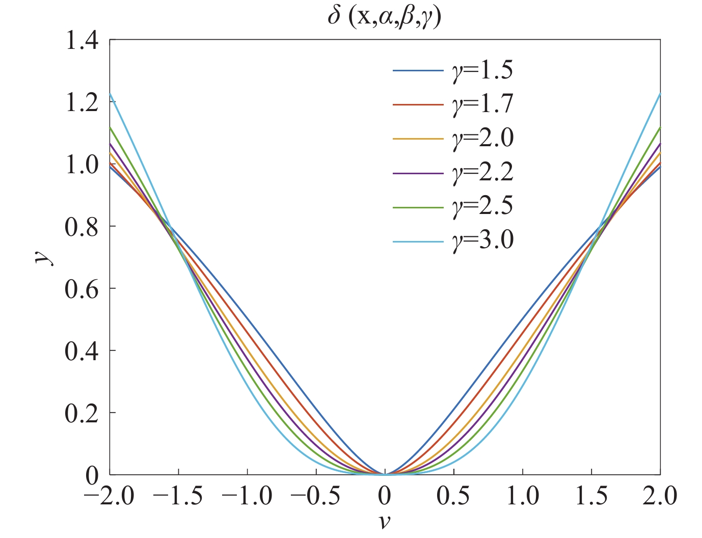
Generalized general robust loss function with different parameters γ.
| Citation: |
Jinhui Hu and Haiquan Zhao, “Adaptive generalized robust iterative cubature kalman filter,” Chinese Journal of Electronics, vol. x, no. x, pp. 1–9, xxxx. DOI: 10.23919/cje.2024.00.221

|
 Hu Jinhui: Jinhui Hu was born in Shaanxi Province, China, in 2001. He received B.E. degree from Chang’ An University, Xi’an, China, in 2022. He is working toward the master’s degree with the field of signal and information processing from the School of Electrical Engineering, Southwest Jiaotong University, Chengdu, China. His current research interests include state estimation and adaptive filtering algorithm. (Email:Jhhu_swjtu@126.com)
 Zhao Haiquan: Haiquan Zhao (Senior Member, IEEE) was born in Henan Province, China, in 1974. He received the B.S. degree in applied mathematics, and the M.S. and Ph.D. degrees in signal and information processing from Southwest Jiaotong University, Chengdu, China, in 1998, 2005, and 2011, respectively. Since 2012, he has been a Professor with the School of Electrical Engineering, Southwest Jiaotong University. From 2015 to 2016, as a Visiting Scholar, he worked with the University of Florida, USA. His current research interests include information theoretical learning, adaptive filter, adaptive network, active noise control, Kalman filter, machine learning, and artificial intelligence. Dr. Zhao is the author or coauthor of more than 200 international journal papers (SCI indexed), and the owner of 70 invention patents. Prof. Zhao has won several provincial and ministerial awards, and many best paper awards of international conferences or IEEE Transactions. He has served as an Active Reviewer for several IEEE transactions, IET series, signal processing, and other international journals. At present, he is a Handling Editor of Signal Processing, and also an Associate Editor of IEEE Open Journal of Signal Processing, and IEEE Sensors Journal. (Email: hqzhao_swjtu@126.com)
In this paper, an Adaptive Generalized Robust Iterative Cubature Kalman filter (AGRICKF) is developed to solve the problem of non-Gaussian noise and nonlinear problem employed in state estimation. The general robust loss function (GRL) can adjust the shape of the kernel in real time according to the noise environment, but its performance is still degraded when facing more complex noise environments such as Laplace noise. Therefore, a generalized GRL is further constructed by adding a shape modifier to further modify the shape of the kernel according to the noise environment, so as to effectively improve the ability of the algorithm to face complex noise environments. And the accuracy of the algorithm in nonlinear state estimation problems is enhanced through constructing nonlinear augmented model ensemble prediction error and measurement error. The experimental results confirm that the algorithm proposed in this paper has stronger robustness.
Kalman filter (KF) is a commonly used tool in state estimation problems. The KF is utilized in numerous fields including power systems [1], vehicle navigation [2], and radar tracking [3], etc. While the traditional KF is developed for linear systems [4], various variants of KF such as extend Kalman filter (EKF) [5], unscented Kalman filter (UKF) [4], [6] and cubature Kalman filter (CKF) [7], [8] are further developed for nonlinear systems [4].However, with the increasing nonlinearity of the system, it is difficult to obtain good state estimation results with the traditional nonlinear KF variant. Therefore, iterative algorithms such as iterative EKF [9], [10], iterative UKF [11] and iterative CKF [12], [13] etc are developed to further enhance the performance of KF when dealing with nonlinear systems. In addition, different algorithms have been proposed to improve the accuracy of nonlinear state estimation.
Various types of non-Gaussian noise problems in the observations can occur due to various failures that may occur in the sensors during the state estimation process, such as sudden changes in the measurements due to sensor damage. However, the KF and its nonlinear variants using the Minimum Mean Square Error (MMSE) criterion leads to a degradation of the filter’s performance in the face of non-Gaussian noise situations and do not allow for accurate state estimation [11].In order to address this problem, various variants of KF have been proposed in existing research using different robust criteria instead of MMSE. Among them, the Maximum Correntropy Criterion (MCC) [14] as well as the Minimum Error Entropy (MEE) criterion [4] have been used to replace the MMSE criterion to optimize the KF to develop the Maximum correntropy Kalman filtering (MCKF) [15] and Minimum Error Entropy Kalman Filter (MEEKF) [16] due to their strong performance in the face of non-Gaussian noise environments. Furthermore, the MCKF and MEEKF are improved so that the two algorithms can be applied to more complex systems and noisy environments [17] [18]. For instance, to investigate systems with state saturation as well as stochastic nonlinear systems, C-MCKF [19] is developed to solve the problem. And there is also iterative MCUKF [11] and improve iterative MCCKF [20] developed for nonlinear systems. In addition, the strong performance of M-estimation cost functions to deal with non-Gaussian noise is also noted, where cost functions such as Huber, Cauchy, Welsch, etc., show excellent performance in dealing with non-Gaussian noise. Various robust Kalman filters, such as Huber-UKF [21] M-estimation-based MCKF [22], Outlier Robust Iterative EKF [10], and so on [23], have been developed using the M-estimation cost function. Moreover, the impressive efficacy of a general robust loss function [24] has been widely used in the arenas of deep learning, state tracking, and image recognition [24], [25]. It adjusts the shape of the core in real time to the noise environment. And it can cope with complex noise environments relative to the general M-estimation cost function. However, its single kernel parameter tuning still leads to degradation of the algorithm’s performance when faced with more complex noise distribution.
Therefore, for various types of non-Gaussian noise problems caused by sensors damage and so on, in this paper, we improve the general robust loss function to propose a new generalized general robust loss function. And further considering the nonlinear state estimation problem of the robust Kalman filtering algorithm, an Adaptive Generalized Robust Iterative Cubature Kalman filter (AGRICKF) is then proposed. The main contributions of this paper are as follows
1. A new generalized general robust loss function is proposed by adopting a shape modification parameter on the basis of the general robust loss function, which effectively cope with more complex noise distributions.
2. An adaptive generalized robust iterative cubic Kalman filter (AGRICKF) is proposed. The algorithm can effectively handle non-Gaussian noise in state estimation as well as nonlinear state estimation problems. And an adaptive method for the parameters of the algorithm is given.
3. The experimental results validate the performance of the proposed algorithm.
The rest of the article is organized as follows. In Section 2 we give the form of the generalized general robust loss function. The main steps of the Adaptive Generalized Robust Iterative Cubature Kalman filter and parameter optimization are given in Section 3. The results of the experiments are given in Section IV and finally the conclusions are drawn in Section V.
Before proposing the generalized general robust loss function, we first review the general robust loss function, which has the following general form [24], [25]
| δ(v,α,β)=|α−2|α[((v/β)2|α−2|+1)α/2−1] | (1) |
When α is the shape parameter that determines the robustness of this function. When α=2, it is L2 loss; when α=0, it becomes Cauchy; when α=−2, it becomes Geman-McClure loss; and when α=−∞, it is Correntropy induced. β is then a proportionality parameter that controls the size of the loss quadratic bowl for errors near 0. Considering that a single parameter tuning does not allow the cost function to face more complex noise distributions, the generalized general robust loss function is defined as:
| δ(v,α,β,γ)=|α−γ|α[(|v/β|γ|α−γ|+1)αγ−1] | (2) |
where γ is a shape modification parameter, which is further extended to make the loss function more effective in achieving better performance in more complex noise environments. When γ=2, the loss function degenerates to an ordinary general robust loss function. And our proposed cost function also has the scalability of a general robust loss function, which takes the following form for different values of α for the generalized general robust loss function.
| δ(v)={m∑i=1log(1γ|vi/β|γ+1),α=0m∑i=12(1−(|vi/β|γ2γ+1)−2),α=−γm∑i=1(1−exp(−1γ|vi/β|γ)),α=−∞m∑i=1|α−γ|α((|vi/β|γ|α−γ|+1)α/γ−1),otherwise | (3) |
To further illustrate the advantages of our proposed cost function over general robust loss functions, we compare the shapes of the cost function and its gradient for different parameter γ.As can be seen in Figure 1 and Figure 2, the shape of the function and its gradient changes when the parameter γ takes on different values. Figure 1 and Figure 2 show that when the size of the error and the parameter α are determined, further adjustment of the parameter γ will make the size of the weight on the error change further, thus achieving a more flexible weighting for the error point. Therefore, when facing more diversified noise problems, our proposed cost function will be handled more flexibly, so that the robust Kalman filtering algorithm we obtained using this cost function will cope with more complex noise environments.
Remark 1: Although general robust cost function can be adapted to different noise distributions by changing the kernel parameter α, it still leads to degradation of the cost function’s performance when confronted with more complex noise distributions. Therefore, the shape factor γ is further introduced to modify the kernel shape rather than changing alone, which better enable the cost function to cope with different distributions of noise types.
Remark 2: For different noise distributions to be processed, the generalized general robust loss function will assign different weights to the errors at different time points, and when all the parameters are determined, the size of the weights is determined by the error size. However, the rule of weighting only according to the error size is often difficult to perform optimally when facing various types of noise distributions with different distributions in the filter. Therefore, when confronted with different noise distributions, by continuously adjusting the shape parameters to find the optimal weights to assign to the error points, the performance of the filter will be effectively improved.
In this subsection, a new Adaptive Generalized Robust Iterative Cubature Kalman filter (AGRICK) is given. And the shape parameters of the Generalized general robust loss function are determined.
Consider the following nonlinear system state model
| vt=f(vt−1)+wt−1, | (4) |
| zt=g(vt)+rt, | (5) |
where vt and zt represent n-dimensional and m-dimensional state vectors and observation vectors, respectively. f(⋅) and g(⋅) represent the state transfer function and observation function, respectively. wt−1 and rt are the state noise and observation noise with covariance matrices Wt−1 and Rt, respectively, that have zero mean and are uncorrelated. Considering the CKF algorithm has a higher desired accuracy as well as a moderate computational cost [8]. Therefore, the CKF is used to compute the priori state estimates ˆvt|t−1 and the priori covariance matrix Pt|t−1. Letting Pt−1=Σt−1ΣTt−1.
Calculating Sampling Points:
| θt−1(k)=Σt−1η(k)+vt−1, | (6) |
where
| η(k)={√na(k),k=1,2,…,n−√na(k),k=n+1,n+2,…,2n | (7) |
where a(k) denotes the vector whose k-th element is 1 and other elements are 0. Next, calculate the cubature points after the transfer
| ξt|t−1(k)=f(θt−1(k)),k=1,2,…,2n. | (8) |
Calculate the predicted states and the a priori covariance matrix
| ˆvt|t−1=12n2n∑k=1ξt|t−1(k), | (9) |
| Pt|t−1=12n2n∑k=1ˆξt|t−1(k)ˆξTt|t−1(k)+Wt−1. | (10) |
Then an augmentation model is constructed to fuse the prediction error with the measurement error. The model is as follows [10], [11]
| [ˆvt|t−1zt]=[vtg(vt)]+Qt, | (11) |
where
| Qt=[−(vt−ˆvt|t−1)rt]. | (12) |
Easily we can get
| E[QtQ⊤t]=[Upt|t−1(Upt|t−1)⊤00Urt(Urt)⊤]=UtU⊤t, | (13) |
where Ut, Upt|t−1 and Urt are obtained by Cholesky decomposition of E[QtQ⊤t], Pt|t−1 and Rt, respectively. By left-multiplying (11) by U−1t, we get
| Δt=D(vt)+et, | (14) |
where
| Δt=U−1t[ˆvt|t−1zt], | (15) |
| D(vt)=U−1t[vtg(vt)], | (16) |
| et=U−1tQt. | (17) |
It suggests that E[ete⊤t]=In+m. According to (1), the cost function of GRKF is
| δ(vt)=1n+mn+m∑i=1|α−2|α((|et(i)|/β|γ|α−2|+1)α/γ−1), | (18) |
where et(i) represents the i-th element of et. Then the optimal value of the state is obtained by minimizing (18).
| ˆvt=argminvtδ(vt)=argminvt1n+mn+m∑i=1|α−γ|α×((|et(i)|/β|γ|α−γ|+1)α/γ−1)(∂et(i)∂vt). | (19) |
To find the gradient of the cost function, we have
| ∂δ(vt)∂vt=1n+mn+m∑i=1|et(i)|γ−2|β|γ×((|et(i)|/β|γ|α−γ|+1)α/γ−1et(i)∂et(i)∂vt). | (20) |
Then consider the following diagonal matrix
| Ξ(et)=[Ξv(et)00Ξz(et)], | (21) |
where
| Ξv(et)=diag[ψ(et,1),ψ(et,2),…,ψ(et,n)], | (22) |
| Ξz(et)=diag[ψ(et,n+1),ψ(et,n+2),…,ψ(et,n+m)], | (23) |
where ψ(et,n+1)=|et,n+1(i)|γ−2|β|γ(|et,n+1(i)/β|γ|α−γ|+1)α/γ−1, and diag(⋅) represents the transformation of a vector into a diagonal matrix. Letting St=∂et∂vt., (20) can be written as
| ∂δ(vt)∂vt=−S⊤tΞ(et)(Δt−D(vt)). | (24) |
Making the gradient equal to 0, we have
| vi+1t=vit−(S⊤t,iΞ(eit)St,i)−1S⊤t,iΞ(eit)(Δt−D(vit)), | (25) |
where i represents iteration index. According to the matrix inversion lemma [15], [16], one can obtain
| ˆvit=ˆvt|t−1+Git(zt−g(ˆvit)−Bit(ˆvt|t−1−ˆvit)), | (26) |
where
| Bit=∂g∂vt|vt=vit, | (27) |
| Git=¯Pit|t−1(Bit)⊤(vit)(Bit¯Pit|t−1(Bit)⊤(vit)+¯Rit), | (28) |
| ¯Pit|t−1=Upt|t−1(Ξv(eit))−1(Upt|t−1)⊤, | (29) |
| ¯Rit=Urt(Ξz(eit))−1(Urt)⊤. | (30) |
The posterior covariance matrix is then updated by
| Pt=(In−GtBit)¯Pt|t−1. | (31) |
Remark 3: The generalized general robust loss function used in our proposed AGRICKF algorithm cope with more complex noise distributions, and the algorithm degenerates to Adaptive Robust Iterative Cubature Kalman filter (ARICKF) when the shape parameter γ=2.
Remark 4: The AGRICKF algorithm proposed in this paper processes the noise at each moment when confronted with measurements containing Gaussian noise as well as non-Gaussian noise. Although the filter may not have fully processed the error at the previous moment, resulting in the state estimation results still not accurate enough. However, the construction of the error generalization model in (11) helps the filter to process the state error in real time as well, and although there is a certain amount of accumulated error, the accumulated error will continue to be processed at the next moment, which will help the filter’s state estimation error to become smaller and smaller, thus achieving the convergence of the error behavior.
| Algorithm 1 AGRICKF |
| Require: f(⋅), g(⋅), Wt, Rt, ε, a, β |
| 1: Input:vt|t for t=1,2,…,N |
| 2: Initialization: Setting initial filter state values v0|0 and initial covariance matrix values P0|0. |
| 3: for t=1,2,…,N do |
| 4: The priori state estimates vt|t−1 and the priori covariance matrix Pt|t−1 are computed by (6)-(10). |
| 5: while ‖ do |
| 6: Compute the v_{t}^{i+1} via (26). |
| 7: end while |
| 8: Updating the covariance matrix by (31). |
| 9: end for |
Since the parameter \alpha and \gamma determines the shape of the kernel of the general robust loss function. In this subsection, we discuss the optimal values of the parameter \alpha and \gamma. Consider \alpha and \gamma as additional location parameters to minimize the generalized loss.
| \begin{aligned} \left( \hat{{\bf{v}}}, \hat{\alpha}, \hat{\gamma} \right) = \arg\min_{(\alpha, \gamma, {\bf{v}})} \sum_{i=1}^{n+m} \delta \left( e_t(i), \alpha, \beta, \gamma \right). \end{aligned} | (32) |
A value of \alpha and \gamma can be obtained using (32), but this value of \alpha essentially minimizes all errors without affecting {\bf{v}}, i.e., treating all data as outliers. To avoid this, a generalized loss function [24] is constructed by
| \begin{aligned} P(e, \alpha, \beta, \gamma) = \frac{1}{\beta L(\alpha)} \exp\left(-\delta(e, \alpha, \beta, \gamma)\right), \end{aligned} | (33) |
where
| \begin{aligned} L(\alpha, \gamma) = \int_{-\theta}^{\theta} \exp\left(-\delta(e_t, \alpha, 1, \gamma)\right) de_t, \end{aligned} | (34) |
where \theta is the truncation limit of the approximate integral. The optimal value of the parameter \alpha can then be obtained by minimizing the negative logarithm of the generalized loss function.
| \begin{aligned} \left( \hat{\alpha}, \hat{\gamma} \right) = \arg\min_{(\alpha, \gamma, {\bf{v}})} -\sum_{i=1}^{n+m} \log\left( P(e, \alpha, \beta, \gamma) \right). \end{aligned} | (35) |
Remark 5: During the experiment, the algorithm does not work when the parameter \alpha is larger than 1, and the effect on the performance of the algorithm is not obvious when the parameter \alpha is smaller than -10. And due to the gradient calculation is very complicated, the optimal values of the algorithm parameters \alpha and \gamma are determined by using a grid search, the optimization range are set to [-10, 1] with a resolution of 0.1 and [1.5, 2.5] with a resolution of 0.01, respectively.
In this section, we analyze the error behavior of AGRICKF and give the convergence analysis of AGRICK’s mean error behavior and mean square error behavior, respectively.
First define the error of the posteriori state estimation
| \begin{aligned} \sigma_t = {\bf{v}}_t - \hat{{\bf{v}}}_{t|t}. \end{aligned} | (36) |
According to (4), (5), (26), (36) can be written as
| \begin{aligned} \sigma_t = \left( {\bf{I}}_n - {\bf{G}}_t {\bf{B}}_t \right) {\bf{F}} \sigma_{t-1} + \left( {\bf{I}}_n - {\bf{G}}_t {\bf{B}}_t \right) {\bf{w}}_t - {\bf{G}}_t {\bf{r}}_t. \end{aligned} | (37) |
Since {\bf{w}}_t and {\bf{r}}_t are both noisy with mean 0. Therefore, the mathematical expectation of the \sigma_t is
| \begin{aligned} E[\sigma_t] = ({\bf{I}}_n - {\bf{G}}_t {\bf{B}}_t) {\bf{F}} E[\sigma_{t-1}]. \end{aligned} | (38) |
Since the state transfer function {\bf{f}}(\cdot) and the measurement function {\bf{g}}(\cdot) in the state-space equations considered in this paper are both time-invariant, both {\bf{F}} and {\bf{B}}_t are stable. According to (20)-(30), and since
| \begin{split} & \psi(e_{t,n+1}) \\&= \frac{|e_{t,n+1}(i)|^{\gamma-2}}{|\beta|^\gamma} \left( \left| \frac{e_{t,n+1}(i)}{\beta} \right|^\gamma / |\alpha - \gamma| + 1 \right)^{\alpha/\gamma - 1}, \end{split} | (39) |
which is a positive definite matrix, the Kalman gain {\bf{G}}_t is stable.
Further considering the mean square error behavior of AGRICKF, the error covariance matrix of the algorithm is first given
| \begin{split} E\left[\sigma_t \sigma_t^\top\right] = \;&\left({\bf{I}}_n - {\bf{G}}_t {\bf{B}}_t\right) {\bf{F}} E\left[\sigma_{t-1} \sigma_{t-1}^\top\right]\\& {\bf{F}}^\top \left({\bf{I}}_n - {\bf{G}}_t {\bf{B}}_t\right)^\top + \ell_t, \end{split} | (40) |
where
| \begin{aligned} \ell_t = \left( {\bf{I}}_n - {\bf{G}}_t {\bf{B}}_t \right) {\bf{W}}_t \left( {\bf{I}}_n - {\bf{G}}_t {\bf{B}}_t \right)^\top + {\bf{G}}_t {\bf{R}}_t {\bf{G}}_t^\top. \end{aligned} | (41) |
Letting
| \begin{aligned} \hbar_t = \left( {\bf{I}}_n - {\bf{G}}_t {\bf{B}}_t \right) {\bf{F}}, \end{aligned} | (42) |
| \begin{aligned} \lambda_t = E\left[ \sigma_t \sigma_t^\top \right]. \end{aligned} | (43) |
(39) can be rewritten as
| \begin{aligned} \lambda_t = \hbar_{t} \lambda_t \hbar_{t}^T + \ell_{t}. \end{aligned} | (44) |
Similarly, since the noise covariance matrices {\bf{W}}_t and {\bf{R}}_t of the Kalman filtering algorithm are set invariant in advance, and the algorithm in this paper does not take into account the case where {\bf{W}}_t and {\bf{R}}_t are unknown. Thus \hbar_t and \ell_t are time-invariant, so the error covariance matrix \lambda_t of the algorithm converges. We give the limiting case of (44)
| \begin{aligned} \lim_{t \to \infty} \lambda_t = \lim_{t \to \infty} \hbar_{t} \lambda_{t-1} \hbar_{t}^\top + \lim_{t \to \infty} \ell_t. \end{aligned} | (45) |
Letting \lim_{t \to \infty} \lambda_t=\lambda, \lim_{t \to \infty} \hbar_{t}=\hbar, \lim_{t \to \infty} \ell_t= \ell. We simplify (45) to a real discrete time Lyapunov equation
| \begin{aligned} \lambda=\hbar \lambda \hbar^T + \ell, \end{aligned} | (46) |
with
| \begin{aligned} \text{vec}(\lambda) = \left( {\bf{I}} - \hbar \otimes \hbar ^\top \right)^{-1} + \text{vec}(\ell). \end{aligned} | (47) |
where \otimes represents the Kronecker product.
At this point, we can conclude that the mean square error behaviour of the proposed algorithm AGRICKF converges and the proposed algorithm is stable.
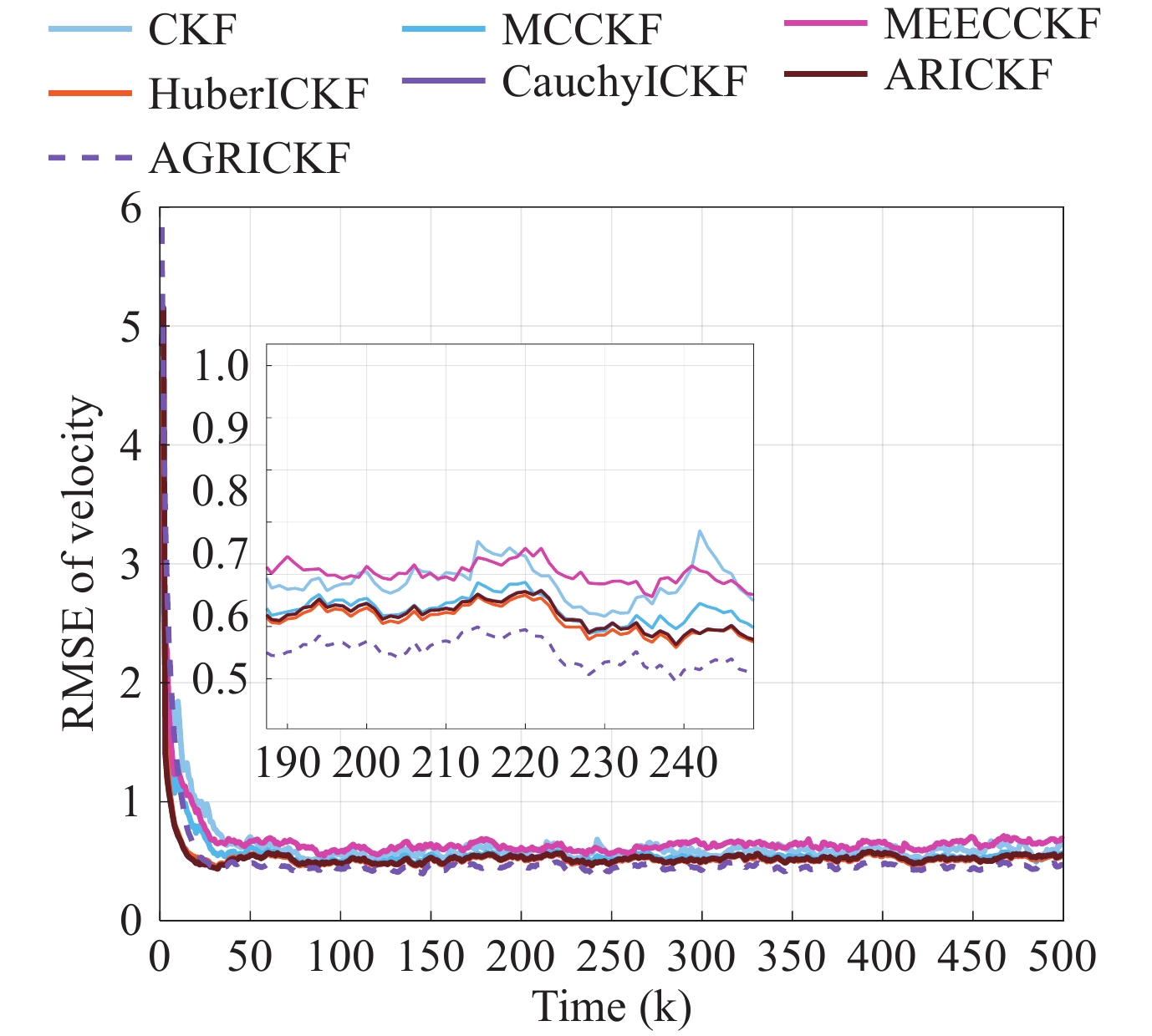
In this section, the performance of the proposed AGRICKF algorithm is validated. The robustness of AGRICKF is demonstrated through comparison with CKF [7], ICKF, MCCKF [15], MEECKF [16], HuberICKF [10], CauchyICKF [10] and ARICKF. The iterative convergence threshold was set to. The kernel width those are set in Table I. To enhance the statistical characterization of the experimental outcomes, we executed M=100 independent Monte Carlo experiments. RMSE is used as metrics for performance comparison. RMSE is defined as
| \begin{aligned} \text{RMSE}(t) = \sqrt{\frac{1}{M} \sum_{k=1}^{M} \left( \left\| {\bf{v}}_t^k - \hat{{\bf{v}}}_t^k \right\|^2\right)}. \end{aligned} | (48) |
where {\bf{v}}_t^k and \hat{{\bf{v}}}_t^k represents the true state and estimated state value at t-th moment and k-th Monte Carlo experiments.
Considering the following nonlinear Land Vehicle Navigation system [16]
| \begin{aligned} {\bf{v}}_t = \begin{bmatrix} 1 & 0 & T & 0 \\ 0 & 1 & 0 & T \\ 0 & 0 & 1 & 0 \\ 0 & 0 & 0 & 1 \end{bmatrix} {\bf{v}}_{t-1} + {\bf{w}}_{t-1}, \end{aligned} | (49) |
| \begin{aligned} {\bf{z}}_t = \begin{bmatrix} -{\bf{v}}_t(1) - {\bf{v}}_t(3) \\ -{\bf{v}}_t(2) - {\bf{v}}_t(4) \\ \sqrt{{\bf{v}}_t^2(1) + {\bf{v}}_t^2(2)} \\ \arctan \left( \dfrac{{\bf{v}}_t(1) + 100}{\sqrt{{\bf{v}}_t(2) + 100}} \right) \end{bmatrix} + {\bf{r}}_{t-1}, \end{aligned} | (50) |
where {\bf{v}}_t = \begin{bmatrix} v_{t}(1) & v_{t}(2) & v_{t}(3) & v_{t}(4) \end{bmatrix}^\top is state vector consisting of the north position, the east position, the north velocity and the east velocity. T=0.1 is the sampling interval. The real state value, the initial state value, and the initial covariance matrix are set as {\bf{v}}_0 = \begin{bmatrix} 0 & 10 & 5 & 10 \end{bmatrix}^\top, {\bf{v}}_{1|0} = \begin{bmatrix} 1 & 1 & 1 & 1 \end{bmatrix}^\top, {\bf{P}}_{1|0}={\bf{eye}}(n).
| Kernel width | Threshold \varepsilon | |
| MCCKF | 25 | 10^{-6} |
| MEECKF | 2 | 10^{-6} |
| HuberICKF | 1.345 | 10^{-6} |
| CauchyICKF | 1.345 | 10^{-6} |
 DownLoad:
CSV
DownLoad:
CSV
Case A Impact of parameters
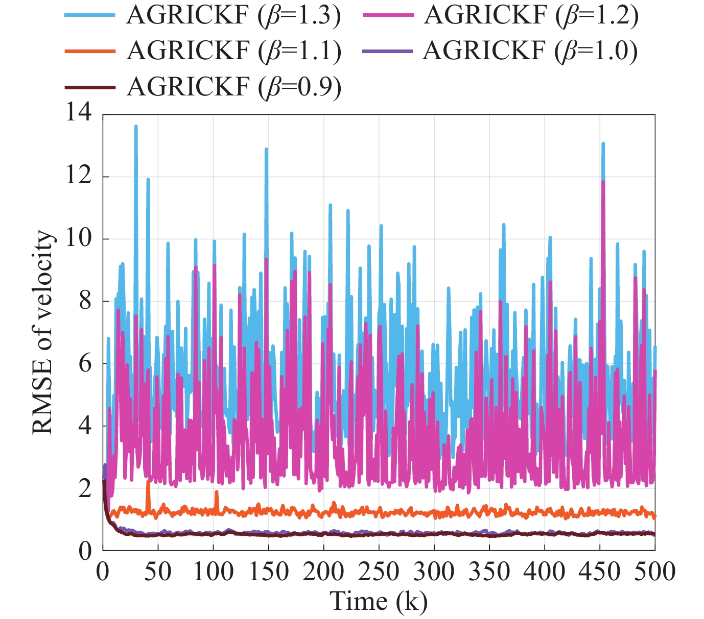
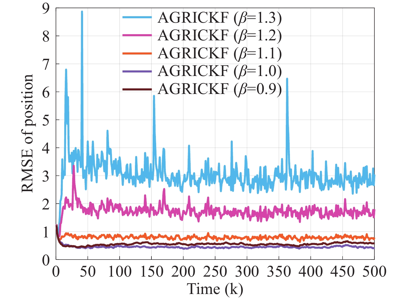
We begin by evaluating the AGRICKF parameters in the scenario of Gaussian noise with random outliers, and assess the RMSEs with varying parameters. As the observer of the navigation system receives various types of non-Gaussian noise, such as anomalous data, loss of observation data, etc. We use a mixture of two Gaussian noises to simulate the possible non-Gaussian noise problem in this section. The Gaussian distribution with large variance is used to simulate the possible outlier data, and the Gaussian distributed noise with a smaller variance is used to model the interference of the measurements by various types of environmental noise during transmission. The noise of Gaussian noise with random outliers is given by
| \begin{aligned} {\bf{r}}_t=0.01N(0,1000)+0.99N(0,1), \end{aligned} | (51) |
where N(a,b) represents Gaussian noise with a mean of a and a variance of b. The process noise is setting to {\bf{w}}_t=N(0,0.01). In Figure 3 and Figure 4, the RMSE for different values of \beta is compared. It can be concluded that the value of \beta has a large impact on the accuracy of the algorithm, and when obtains a suitable value, it can make our algorithm have better robustness. In subsequent experiments, we set \beta=1.0.
In addition, the performance of the algorithm is compared for different values of the parameters \alpha and \gamma in order to validate our proposed method of adaptive parameter selection. \text{ARMSE}=\frac{1}{N}\sum_{t=1}^{N} \text{RMSE}(t) is used as the evaluation index, where N is total time steps, and the comparison results are shown in Table II. It can be seen that the use of adaptive parameter selection helps the filter to achieve more accurate estimation results, which is due to the fact that the optimal parameters in this noisy environment are found by this method, effectively eliminating the influence of outliers.
| (\alpha,\gamma) | ARMSE of position | ARMSE of velocity |
| adaptive parameter | ||
| (0,2.0) | ||
| (0,2.1) | ||
| (0,2.15) | ||
| (0,2.2) | ||
| (-2,2.1) | ||
| (1,2.1) | ||
| (2,2.1) |
DownLoad:
CSV
Case B Algorithm Robustness Comparison
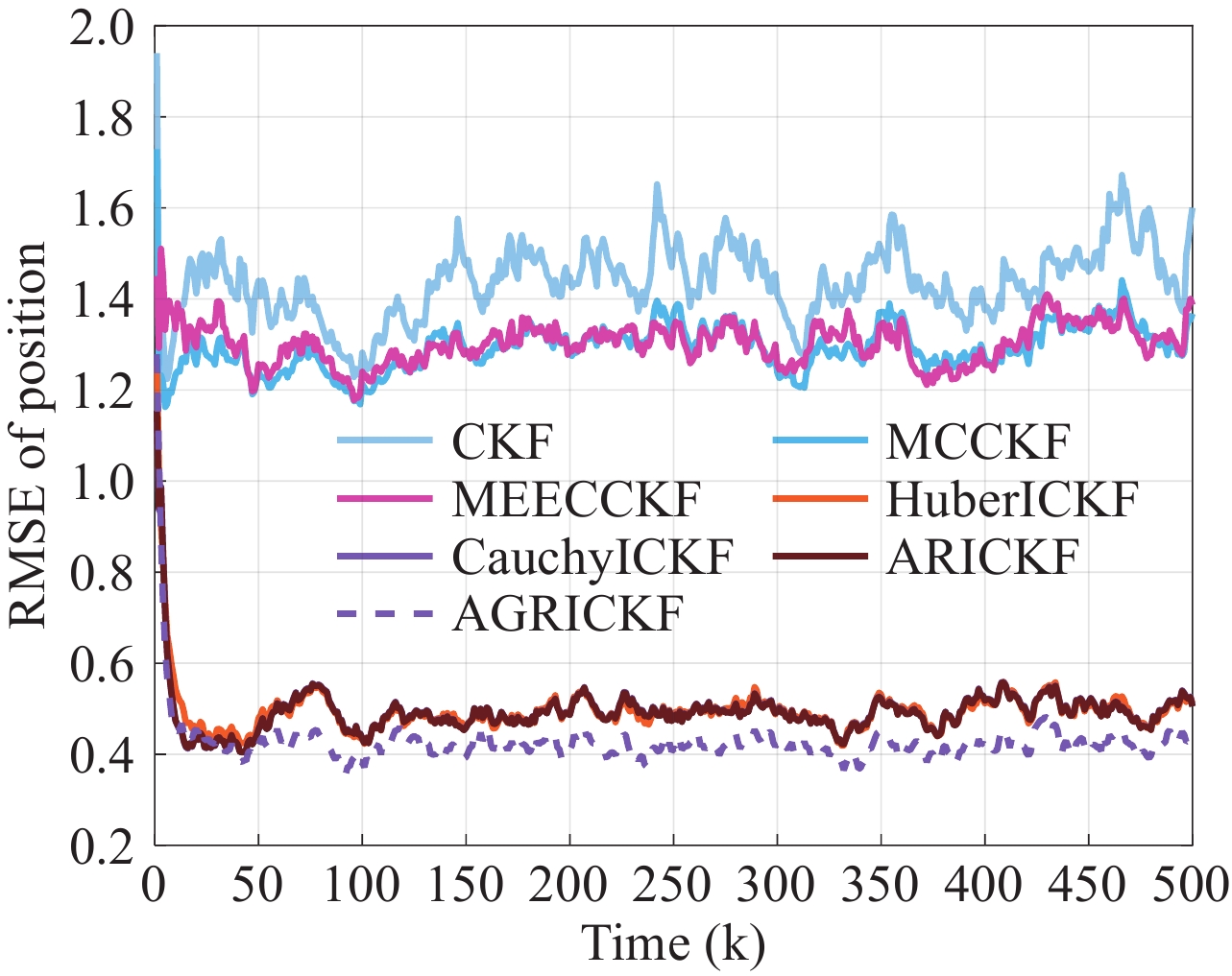
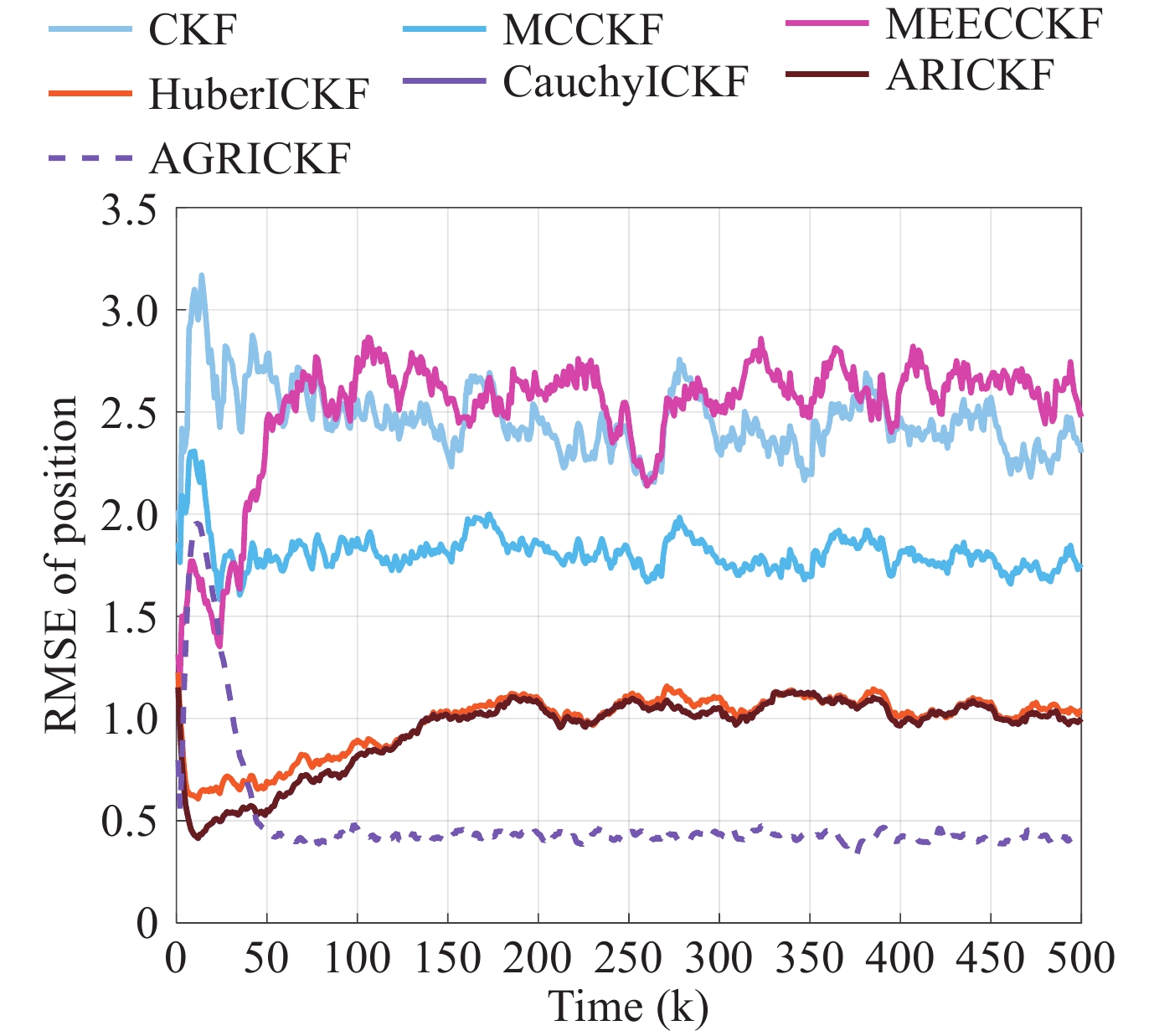
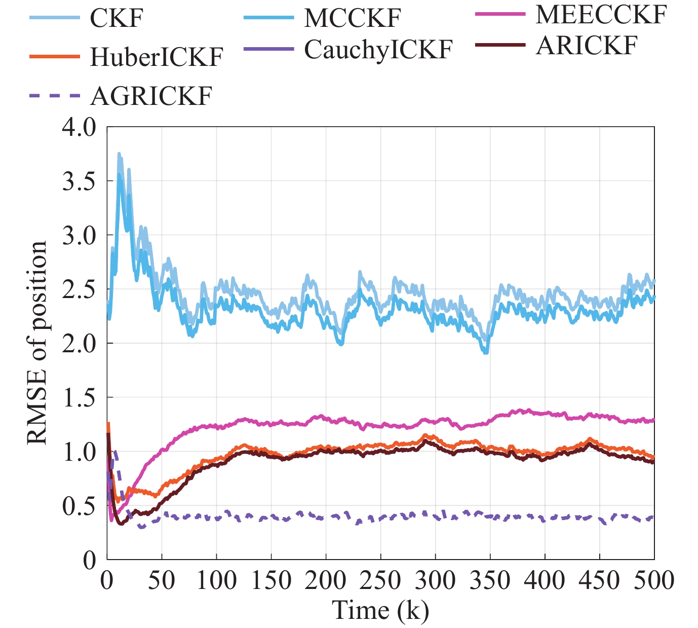
In this subsection, the enhanced robustness of our proposed AGRICKF algorithm is demonstrated through comparison with other robust algorithms. The process noise setting is still Gaussian noise, the same as Case A. A Gaussian mixture model is also used to model possible non-Gaussian noise problems. However, in this section the noise of the Laplace distribution is used to model the appearance of outliers. The algorithm is tested separately using the following two noisy environments.
| \begin{aligned} {\bf{r}}_{1,t}=0.8N(0,1)+0.1N(-1,1000)+0.1N(1,1000), \end{aligned} | (52) |
| \begin{aligned} {\bf{r}}_{2,t}=0.01L(0,1000)+0.99N(0,1), \end{aligned} | (53) |
| \begin{aligned} {\bf{r}}_{3,t}=0.01L(100,1000)+0.99N(-0.1,1), \end{aligned} | (54) |
where L(0,1000) represents Laplace noise with a mean of 0 and a variance of 1000. Figure 5-10 show the RMSE in these three environments respectively. It is clearly concluded that our proposed AGRICKF algorithm exhibits superior robustness and maintains strong performance in a variety of complex noise environments. Thus, in the same way as the theoretical analysis, the AGRICKF shows a strong performance when dealing with complex non-Gaussian noise problems.
In this paper, an iterative Cubature Kalman filter based on a generalize general robust loss function (AGRICKF) is developed. As the generalize general robust loss function used can be converted into multiple M-estimation functions, the AGRICKF algorithm can handle various complex non-Gaussian noise environments. And the algorithm constructs a nonlinear augmented model ensemble of prediction errors and measurement errors to improve the accuracy of the algorithm in the face of nonlinear state estimation problems. The experimental results confirm the impact of the algorithm parameters and its enhanced robustness compared to other robust algorithms.
This work was supported by National Natural Science Foundation of China (grant:
| [1] |
H. Q. Zhao and B. Y. Tian, “Robust power system forecasting-aided state estimation with generalized maximum mixture correntropy unscented Kalman filter,” IEEE Transactions on Instrumentation and Measurement, vol. 71, article no. 9002610, 2022. DOI: 10.1109/TIM.2022.3160562
|
| [2] |
T. Basar, “A new approach to linear filtering and prediction problems,” in Control Theory: Twenty-Five Seminal Papers (1932–1981), T. Başar, Ed. IEEE Press, New York, NY, USA, pp. 167–179, 2001.
|
| [3] |
Y. M. Zhang, M. G. Amin, and F. Ahmad, “Application of time-frequency analysis and Kalman filter to range estimation of targets in enclosed structures,” in Proceedings of 2008 IEEE Radar Conference, Rome, Italy, pp. 1–4, 2008.
|
| [4] |
B. D. Chen, L. J. Dang, N. N. Zheng, et al., Kalman Filtering Under Information Theoretic Criteria. Springer, Cham, Germany, 2023.
|
| [5] |
X. D. Liu, L. Y. Li, Z. Li, et al., “Stochastic stability condition for the extended Kalman filter with intermittent observations,” IEEE Transactions on Circuits and Systems II: Express Briefs, vol. 64, no. 3, pp. 334–338, 2017. DOI: 10.1109/TCSII.2016.2578956
|
| [6] |
H. W. Zhang and W. X. Xie, “Constrained unscented Kalman filtering for bearings-only maneuvering target tracking,” Chinese Journal of Electronics, vol. 29, no. 3, pp. 501–507, 2020. DOI: 10.1049/cje.2020.02.006
|
| [7] |
I. Arasaratnam and S. Haykin, “Cubature Kalman filters,” IEEE Transactions on Automatic Control, vol. 54, no. 6, pp. 1254–1269, 2009. DOI: 10.1109/TAC.2009.2019800
|
| [8] |
L. J. Dang, B. D. Chen, Y. L. Huang, et al., “Cubature Kalman filter under minimum error entropy with fiducial points for INS/GPS integration,” IEEE/CAA Journal of Automatica Sinica, vol. 9, no. 3, pp. 450–465, 2022. DOI: 10.1109/JAS.2021.1004350
|
| [9] |
J. B. Zhao, M. Netto, and L. Mili, “A robust iterated extended Kalman filter for power system dynamic state estimation,” IEEE Transactions on Power Systems, vol. 32, no. 4, pp. 3205–3216, 2017. DOI: 10.1109/TPWRS.2016.2628344
|
| [10] |
Y. T. Z. Tao and S. S. T. Yau, 2023, “Outlier-robust iterative extended Kalman filtering,” IEEE Signal Processing Letters, vol. 30, pp. 743–747, 2023. DOI: 10.1109/LSP.2023.3285118
|
| [11] |
H. Q. Zhao, B. Y. Tian, and B. D. Chen, “Robust stable iterated unscented Kalman filter based on maximum correntropy criterion,” Automatica, vol. 142, article no. 110410, 2022. DOI: 10.1016/j.automatica.2022.110410
|
| [12] |
B. B. Cui, X. Y. Chen, Y. Xu, et al., “Performance analysis of improved iterated cubature Kalman filter and its application to GNSS/INS,” ISA Transactions, vol. 66, pp. 460–468, 2017. DOI: 10.1016/j.isatra.2016.09.010
|
| [13] |
Y. H. Wang and D. M. Liu, “Maximum correntropy cubature Kalman filter and smoother for continuous-discrete nonlinear systems with non-Gaussian noises,” ISA Transactions, vol. 137, pp. 436–445, 2023. DOI: 10.1016/j.isatra.2022.12.017
|
| [14] |
Y. Y. Zhu, H. Q. Zhao, X. P. Zeng, et al., “Robust generalized maximum correntropy criterion algorithms for active noise control,” IEEE/ACM Transactions on Audio, Speech, and Language Processing, vol. 28, pp. 1282–1292, 2020. DOI: 10.1109/TASLP.2020.2982030
|
| [15] |
B. D. Chen, X. Liu, H. Q. Zhao, et al., “Maximum correntropy Kalman filter,” Automatica, vol. 76, pp. 70–77, 2017. DOI: 10.1016/j.automatica.2016.10.004
|
| [16] |
B. D. Chen, L. J. Dang, Y. T. Gu, et al., “Minimum error entropy Kalman filter,” IEEE Transactions on Systems, Man, and Cybernetics: Systems, vol. 51, no. 9, pp. 5819–5829, 2021. DOI: 10.1109/TSMC.2019.2957269
|
| [17] |
J. N. Xing, T. Jiang, and Y. S. Li, “q-rényi kernel functioned Kalman filter for land vehicle navigation,” IEEE Transactions on Circuits and Systems II: Express Briefs, vol. 69, no. 11, pp. 4598–4602, 2022. DOI: 10.1109/TCSII.2022.3183617
|
| [18] |
X. X. Fan, G. Wang, J. C. Han, et al., “Interacting multiple model based on maximum correntropy Kalman filter,” IEEE Transactions on Circuits and Systems II: Express Briefs, vol. 68, no. 8, pp. 3017–3021, 2021. DOI: 10.1109/TCSII.2021.3068221
|
| [19] |
B. Shen, X. L. Wang, and L. Zou, “Maximum correntropy Kalman filtering for non-Gaussian systems with state saturations and stochastic nonlinearities,” IEEE/CAA Journal of Automatica Sinica, vol. 10, no. 5, pp. 1223–1233, 2023. DOI: 10.1109/JAS.2023.123195
|
| [20] |
Q. F. Dou, T. Du, L. Guo, et al., “An improved iterative maximum correntropy cubature Kalman filter,” in Proceedings of 2021 China Automation Congress, Beijing, China, pp. 2582–2586, 2021.
|
| [21] |
C. Gao and J. Sun, “Dynamic state estimation for power system based on M-UKF algorithm,” in Proceedings of the 2020 IEEE 4th Conference on Energy Internet and Energy System Integration, Wuhan, China, pp. 1935–1940, 2020.
|
| [22] |
C. Liu, G. Wang, X. Guan, et al., “Robust m-estimation-based maximum correntropy Kalman filter,” ISA Transactions, vol. 136, pp. 198–209, 2023. DOI: 10.1016/j.isatra.2022.10.025
|
| [23] |
Y. T. Z. Tao, J. Y. Kang, and S. S. T. Yau, “Maximum correntropy ensemble Kalman filter,” in Proceedings of the 2023 62nd IEEE Conference on Decision and Control, Singapore, Singapore, pp. 8659–8664, 2023.
|
| [24] |
J. T. Barron, “A general and adaptive robust loss function,” in Proceedings of 2019 IEEE/CVF Conference on Computer Vision and Pattern Recognition, Long Beach, CA, USA, pp. 4326–4334, 2019.
|
| [25] |
N. Chebrolu, T. Läbe, O. Vysotska, et al., “Adaptive robust kernels for non-linear least squares problems,” IEEE Robotics and Automation Letters, vol. 6, no. 2, pp. 2240–2247, 2021. DOI: 10.1109/LRA.2021.3061331
|
Figures(10) / Tables(2)

CJE QR CODE

CIE QR CODE
Copyright © Editorial Office of Chinese Journal of Electronics |
京ICP备12041980号-1 |

| Kernel width | Threshold \varepsilon | |
| MCCKF | 25 | 10^{-6} |
| MEECKF | 2 | 10^{-6} |
| HuberICKF | 1.345 | 10^{-6} |
| CauchyICKF | 1.345 | 10^{-6} |
DownLoad:
CSV
| (\alpha,\gamma) | ARMSE of position | ARMSE of velocity |
| adaptive parameter | ||
| (0,2.0) | ||
| (0,2.1) | ||
| (0,2.15) | ||
| (0,2.2) | ||
| (-2,2.1) | ||
| (1,2.1) | ||
| (2,2.1) |
DownLoad:
CSV